Aligning with Compensators
Transcription:
In this video, I will show you how to use compensators for tolerancing.
The use of the compensators is that for example, if we have some alignment process included in the mounting of the system, which means we do some manual alignment during this setup of the system, then we can use the compensators to kind of simulate the alignment strategy.
And therefore, we get a more realistic tolerancing result compared that we just assumed that all tolerances are just random.
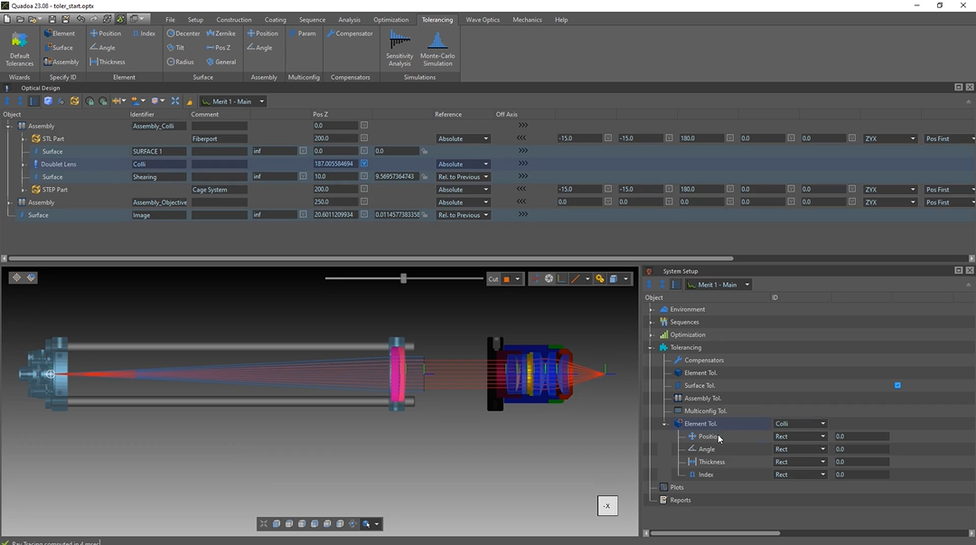
For the demonstration I’ve set up this system, which you can see here.
The rays come here at the left out of the fiber.
This is the assembly, which is collimating, the output of the fiber. So the rays at this point here are collimated.
Afterwards, the rays pass this assembly, which is a microscope objective with which focuses the light on this point here.
For the tolerancing, we assume that the alignment procedure is as follows.
So we set up here this collimator assembly and we have some tolerances there for the tilt and for the d center of the lens.
However, the position along the optical axis in the z direction is manually aligned with a shearing interferometer cube and for that alignment of the optical axis will be very accurate. This means that after applying the tolerances this position in c direction will be aligned so that, the wavefront there is collimated and that the focus term is gone. In the next step after aligning the collimator assembly, the objective lens is mounted in front of the collimator.
The positioning of the lens also has some tolerances and only the defocus will be adjusted manually, which is the second step of the alignment strategy.
So we have two steps. The first step is the alignment of the collimation, and for the second step, the alignment of the defocus of the objective lens.
For this demonstration, we will also ignore the single tolerances inside this assembly of single elements.
So we will only consider the tolerances that are from the whole assembly itself and not from single lenses or surfaces inside the assembly.
What I’ve already prepared is that all elements are already grouped into assemblies.
So you can see here this, collimator assembly and here this microscope objective assembly. And in addition, I set up the pivot points for the assembly.
So if you tilt for example here this microscope objective around here this pivot point in x direction, we will see that it will tilt around the point where it is mounted here and not around the center of gravity.
So this means that these two steps, so the assigning of the assemblies and setting up the pivot points for the assemblies and elements is what has to be always done before starting with the tolerance analysis.
Or the tolerancing we will not use here this tolerance wizard because we only have, these two tolerances here for the collimator assembly and here for, the objective, and therefore it is easier to just set up the tolerances by hand.
For the tolerancing, we will add a new element tolerance.
For that, we just click here on this element.
Now this element tolerance has been added here to the system setup, and there we will assign it to the collimator assembly with the name Collie. You can see here, the name of the the doublet lens here. The identifier name is Collie. We will only take into account the tolerances for the position and for the angle, and therefore, we can delete here thickness and the index.
And the position tolerance is in x y z direction, and the angular tolerance is in tilt in x y direction. The second tolerance we have is the assembly tolerance for the microscope objective, and for that we will add an assembly tolerance.
And as well here, we will assign it to the correct ID name. In our case, it’s assembly, objective.
You can see it here.
And here again, we have a tolerance and angle and in position.
Yeah. And now basically, we have set up the tolerances, and we can continue, in the next step with the compensators. To add the alignment strategy to the tolerancing, we will add a compensator.
I’ve already set up two additional merit functions.
So here this merit function two, is for, the collimator, and this will optimize the sequence with the Blu rays that I’ve set up for this step and will optimize the defocus.
So here you can see that the goal is the defocus and here this additional sequence and with the blue rays is here the sequence two.
Further, we need to assign here, this compensator, to the right metric function. So in our case, it is the defocus collimator merit function.
In the next step, we also need to set the variables for the defocus.
And for that, we go here to the optical design editor.
We select here this compensator.
And for the first compensator, we will align the c position of the doublet lens. So here this, doublet lens, and for that, we will, click here this positions in z direction as a variable.
For the second step of the alignment, we’ll we will add another compensator because the first step of our alignment strategy will first do the defocus compensation of the collimation and afterwards, we will focus the spot.
So first compensator one will be applied and after that compensator two will be applied.
If you have several things which are done in one step you can of course also just add one compensator. So now here for the second compensator we’ll still need to select the correct merit function. So in our case it’s merit function, spot image.
And here you can see the merit function three, which I have selected here for this compensator.
Its goal is here the spot radius.
For the, second compensator, we also need to set the variables. And for that, we select here compensator two. And in our case, we will set the set position of the image surface as variable.
So now we finally set up the compensators and the tolerances, and therefore, we can finally perform the tolerance analysis.
So the first, tolerance analysis will be the sensitivity analysis, which I will perform.
Here for the performance criterion, we need to select, a merit function. In my case, I will just use here this main merit function. That is the merit function that I also use to optimize here my system. But, of course, you can also create another merit function if you would like to use that for, the sensitivity analysis. So now we will click here on okay, and you will see the performance of our system regarding to the tolerance changes.
And as expected, we can see that here the tolerance positions, for the position c of the assembly and for the collimator lens, are almost getting to zero, because these are the ones that get compensated.
We can also perform a Monte Carlo simulation with, for example, one hundred systems. Here again for the performance criterion, I will just select here this main merit function.
Yeah. And here, we can see the distribution of our system regarding to these tolerances, including the compensation.
Yeah. So I hope you learned something new in this video about, setting up compensators.
The download link to the Quadua files for this tutorial will be linked below in the description.
And, yeah, thanks for watching.