Computer Generated Hologram (CGH) Optimization
Learn how to optimize a CGH for interferometric testing of aspheres.
Transcription:
In this video, I will show you how to design a computer generated hologram for the interferometric testing of an aspheric surface.
I’ve already set up some, lenses here.
Here we have the transmission sphere. The transmission sphere generates a spherical wavefront.
On the left side, there will be our interferometer. So the rays come already in a plane wavefront here, at a starting point. Here we have our computer generated hologram. At the moment, it is just a substrate without any phase functions.
So the phase function for the computer generated hologram on the substrate is what we are going to optimize in this tutorial.
The last surface here is our surface under test which is in this case an spherical surface, but of course we could also use a freeform surface.
For the interferometer, we have already set up two sequences.
In the first sequence, which we can see here, is the reference sequence. So here the light goes from the interferometer through the optics and reflects here on the reference surface, which is the FISO cavity surface. From here, it goes back again to the interferometer.
The second sequence is the test sequence, and this sequence goes all the way through the transmission sphere, through the generated hologram, and reflects on the surface on a test and goes back to the interferometer.
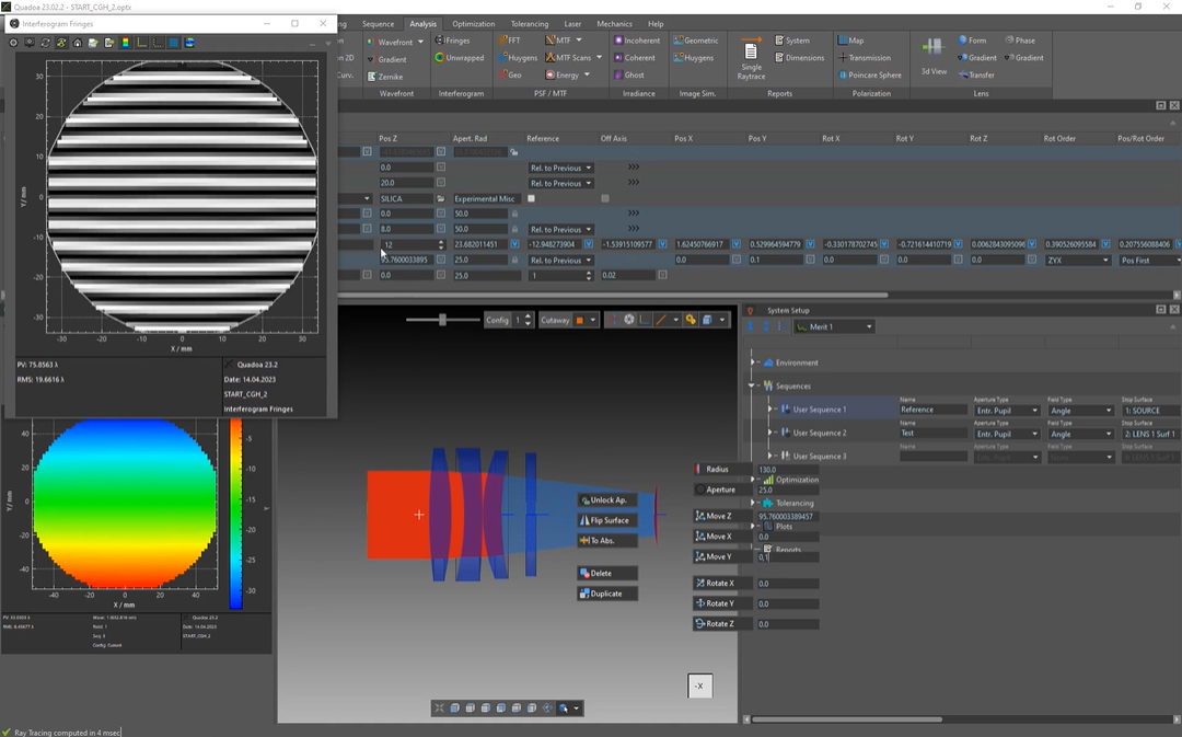
And as you can already see from the rays is that at the moment there’s a large deviation between these two sequences and therefore we cannot evaluate the interferogram at this moment because there are too many fringes here.
So if you check here this interferogram you can see that there are a lot of fringes And for this we will design and optimize the computer generated hologram and it will be used to compensate those fringes.
So let’s start with optimizing the computer generated hologram.
First, I will add a new order sequence. For that, I click here to new order sequence.
I will just hide the first two sequences so that we can see better our third sequence.
We want that the sequence will start from the right and for that, I will revert the sequence direction.
As the source type of the sequence, we will use, wavefront from surface, and the aperture radius is twenty five.
So the same radius as the surface under test.
So here we can see that the rays start perpendicularly from the surface.
And what we need to do is to optimize the phase function of the CDH so we get a plane wavefront on the left side. And for that, the interferogram will work as well.
In the next step, we need to set up the wavelength of the sequence to helium neon, which is the wavelength that we’re using for testing.
The computer generated hologram itself will be added here on the singlet on the second surface here and for that we click with the right mouse button add face and add a radial face function.
The norm radius will be the ray height approximately thirty five millimeters.
For the polynomial order, I will use twelve polynomials to describe the surface.
For the optimization, we will first optimize the absolute wavefront.
So this means that there will be no exit pupil correction in the first step.
For that, we will set up the optical path difference to absolute over image.
For the merit function, we will set a simple merit function that optimizes the wavefront error.
Since we have a high polynomial order, we will increase the grid to fifteen.
And, of course, we need to select the sequence which should be optimized. So in our case, it is the sequence three.
So let’s have a quick look how our wavefront error looks at the moment.
So as we can see here, the main error at the moment is the defocus.
And to get rid of the defocus, we will allow the test surface to align to the right z position to match the basic radius of the transmission sphere wavefront.
So for that, we will optimize here the position of set.
And now we got rid of the defocus and only the spherical aberration is left. In the next step, I will deactivate the variable here of the position set.
And in the second step, I will set all cth coefficients to variable.
In the next step we are now able to optimize and compute here these coefficients and for that we will run again here this local optimization, optimizer.
And as we can see now here these coefficients have been computed. And as we can see here, the wavefront error is zero point zero one, wavelength.
So that’s pretty good, I guess. And if it’s not good enough, of course, we could increase here the number of the polynomial order. Now we can hide here this third sequence and show again here this these first two sequences.
And as you can see, they are matching here pretty good. And when we look here again at our interferogram, we can see that the interferogram is totally black, which means that we have zero fringes.
And maybe we can here tilt a little bit here this surface under test.
And so we can see that it it is basically just a matched computer generated hologram.
Yeah. This was my tutorial about generating computer generated hologram.
Thanks for watching.