Cooke Triplet
Learn how to design a Cooke triplet including setup, optimization, and final iteration.
Transcription:
Hello, and welcome everyone to a new Quadoa tutorial.
Today, we are going to design a classical Cook triplet camera lens from scratch.
Before starting with the actual design, let’s look at the specifications for the lens.
We want the lens to cover the visible wavelength range from around four fifty nanometers to six fifty nanometers.
The field range should be plus minus fifty degrees.
The object is located at infinity.
The entrance pupil diameter should be ten millimeters.
The back focal length should be around fifty millimeters, and the lens materials should be taken from the shot glass catalog. Now in Quadora, we will start from scratch with a new empty file, and the first thing that we will do is to add the three singlet lenses to the design.
For this, we go onto the singlet lens button. We add a singlet lens.
We will start with a basic material, let’s say BK7 from Schott.
And we will duplicate the lens twice, so we have our three lenses.
In the next step, we add two more surfaces to the system.
The first surface is the object space surface, and we will just drag it in front of the first lens up here.
And the second surface is the, image space surface we just added after the last lens. And then we want the back focal length to be fifty millimeters. Therefore, we move it fifty millimeters relative to the last surface of the last lens.
And now as the last step of our setup, we will add some air spaces in between the lenses.
To set up the ray tracing properties, we will change from the optical design editor that we’ve worked in so far to the system setup editor. And here under sequences, we can see our sequence that shows the rays here in red.
And the first thing that we want to change is that the rays do not come here from a point like source, but from infinity.
And this can be achieved by changing the source type to plain wavefront.
Also, we want the entrance pupil diameter to be ten millimeters.
Therefore, we set here the aperture type to entrance pupil, and the aperture radius needs to be to set to five millimeters.
To define the field range that we got from our specification, we go to the field, settings that can be found here in the source, and we will add three more fields.
So we can sample the, field range from zero to fifteen degrees in five degree steps.
As we can see here from the rays, the stop surface is currently located at the second surface of the first lens.
However, for a Cook triplet, typically, the stop surface is located in the center of the whole lens, and therefore, we need to change the position of the stop surface to be at the second lens.
The last thing that we need to do to set up our sequence is to define the wavelength, And this can be done here in the wavelength settings where we can just add the visible wavelength, and we will remove the wavelength that was there in the first place.
In this particular case, as we already know that the result should be something like a Cook triplet, we can precondition the system to notch the optimizer towards that solution.
The easiest way to obtain a good starting system is to interactively pre tune the lenses to obtain something that looks kind of a cooked triplet.
Okay.
Having set up the start system, we can now change to the optimization tab to add a merit function.
To add the merit function, we will use the merit function wizard, and we will just keep all the settings as there are in the default mode and select the spot radius as the main optimization goal.
As variables for the optimization, in the first step, we will allow the curvature of all surfaces to be variable, which can be either achieved by setting the individual surface curvatures to a variable or with this button for the whole system.
To avoid clipping of rays at apertures, as can be seen here, it is typically best practice during optimization to just unlock all the approaches. This means the aperture will directly be computed from the rays that are in the system.
After having everything set up, we can run the optimization. In this case, I will use the local optimizer, and we can just run it. And after about half a second, it’s already finished, and we get our first, result.
We can analyze the spot of the system, and for the first optimization, this already looks pretty good.
One thing that I do not like about this design is that the lenses are a bit bulky.
However, we can easily change this by just adjusting the thickness of the lenses and afterwards running the optimization a second time.
And now this looks a lot cleaner already.
At the moment, the whole system is still made up of three NPK seven lenses.
To optimize the system performance further, we will now allow the optimizer to exchange the lens materials.
To do this, we will first mark all the materials as substitute, and then we will specify the allowed substitute materials.
And for this tutorial, I will just add the whole short catalog to be allowed as a substitute material.
The local optimizer is not capable of optimizing, materials, and, therefore, we will use the extended optimization in this case. And I will also enable the three d view and plot automatic updates so we can see the update of the, performance during the optimization.
Now, of course, we could optimize the system further. However, for this tutorial today, I will consider this as the final design.
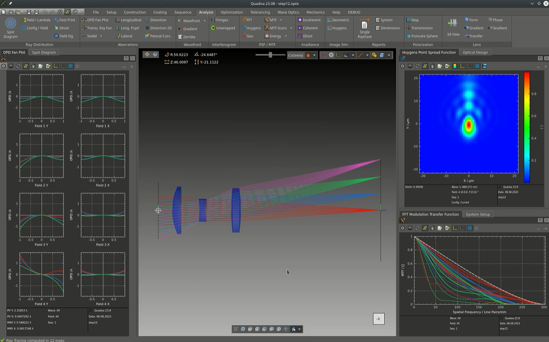
And now we can look at the, system performance.
First, we can open the MTF plot for the system, and we can see that the on axis primary wavelength is close to diffraction limited.
However, for the other fields and also the other wavelength, the performance isn’t that perfect in all cases.
However, for a short example system, this is already pretty good.
And to get a feeling how an image taken with this lens would look like, we can use the geometric image analysis to simulate the image as it would appear on the camera chip.
So I am already at the end of this tutorial.
I hope you learned something new today. And if you want to follow along the steps yourself, we will upload the files, of the models for each step.
See at the link below.