Off-Axis Telescope

Off-Axis Telescope

Learn how to design a parametric off-axis mirror telescope including defining lookup parameters, ray sequence, optimization, analysis of image quality, and export to CAD.

Transcription:

Hello and welcome to this tutorial on the construction of a parametric off axis aspheric mirror telescope. To start with the design, we will start with the primary mirror. And for that, we just add a surface.

We set the identifier to primary.

The next step is we will assign a parabolic form to it, and we will put the quadratic term to zero point zero one.

And we want the aperture to be rectangular and therefore we add a rectangular aperture.

Now we want the model to be parametric, so we also want to parametrically define the aperture. And, therefore, we go here and open the multi config, lookup table.

As you can see, it now appeared here. We’ll just place it besides the, system setup view, And now we can define our parameters.

So the first parameter will be the primary aperture in x direction, and we’ll set this value to forty five.

Now we can use this value to define the aperture in x direction.

As you can see here, the aperture has been applied to the surface.

The next step is to define the aperture in y direction, and this one will be a math equation because we want it to be the aperture in x direction minus a small margin.

We will call it aperture y and the value is aperture x minus the margin. So we haven’t defined the margin yet. This can be done by adding another parameter. We’ll call it margin, and this one will be ten millimeters.

Now, again, we copy the value of the margin and place it over here.

Since we want to have an off axis telescope, we’ll add another, parameter which will be the decentering of the aperture.

And this one will be the center y.

And it’s the, the center plus the margin.

And again, we can apply the center to the surface.

Now, I made a mistake in the beginning. The surface curves into the wrong direction, but we can quickly change this here by adding a minus there.

So the next step is to set up the sequence and, therefore, first, we need an object surface where the light propagates from.

To add the surface, we just add a new surface. We move it before the primary surface.

And now we check that the primary surface is placed here in absolute coordinate space, and therefore, we can move the first surface two hundred millimeters to the left.

Now we do not want the object to be at minus two hundred, but we want the rays to come from infinity.

Therefore, we go to our sequence, to the source setup, and we define the source to be a plane wavefront from infinity.

Also, we want the aperture to be taken from the primary mirror, and we want the, sampling of the aperture to be a grid.

So this can all be set up here in the sequence.

Since we do not need the first surface, we’ll just hide it so it’s not visible in the three d view.

Now the next step is to set up the, secondary surface.

Therefore, again, we add another surface.

We’ll move that one to minus one hundred millimeters, minus two hundred.

And now to make the mirrors bounce off in reflection from this first surface, we need to either add a mirror coating to the surface.

The other option would be to convert the sequence to a user sequence and then define the, order of the surfaces for the rays to be traced.

The secondary mirror also will get a rectangular aperture, and also this one will be parametric. We’ll add two additional parameters for the aperture in x and y.

And we, again, just copy them, or you can also just type the parameter name.

And we’ll make the aperture in x fifteen millimeters and ten in y.

As you can see now, we also need to decenter the aperture.

And for this, we just decenter it by one aperture half size, which is this parameter over here.

Now we can take a look at the three d view. And as we can see here, the ray that is coming from the entrance is a bit vignetted from the, secondary mirror. Therefore, we will increase the margin a bit.

And to be able to get a better sampling here until the border will increase the, sampling of the aperture to a bit more rays.

Now we’ve set up the aperture for the primary and the secondary mirror. And now we want to optimize the form of the secondary mirror to form an image over here where we will add an image plane. So first, we add the image plane.

We will position it in absolute coordinate space at a position of twenty millimeters behind the primary mirror.

And for our sequence to to trace correctly, again, for the secondary mirror, we add, coating, which will be a ideal mirror coating.

Also, we’ll name the secondary mirror and also the image surface.

Now we add a a steric form to the secondary mirror. In this case, I will use a qcon aspheric surface.

And we set the radius as a variable. We allow three polynomial orders, and we will make them all as variables.

The norm radius for this aspugh will be ten millimeters, which is in the range of the aperture.

The next thing to do is to set up the merit function.

In this case, we will just use a default merit function where we will optimize the spot radius without any constraints.

Now over here, we can see, the merit function has been created.

And we have here our variables, which is the curvature as well as the, polynomial terms of the asphere.

And the optimization goal is the spot radius.

Now in the optimization tab, we just click on the local optimizer, and then we let it run.

And after a short time, we directly get, the optimized, surface form.

Now we can see here the aperture of the secondary mirror is a bit too large, which we can quickly fix by changing the aperture size here to eight millimeters in this case.

The next thing that we can do now is to analyze the performance of the telescope. Now what we can do in the analysis tab is we can, look at the spot diagram where we can see this that the system is diffraction limited.

And also the point spread function is already looking good.

Now the next thing that we can do is we can add some fields to our sequence. Therefore, we go here to the, source settings to the fields. We add two more fields and we can enter the, field values for these fields.

We can now also analyze the, point spread function for these different fields.

And we can see that for the third field the point spread function is getting a bit larger, but for the other one it’s pretty close to the ideal case.

Okay. And now we already have our, design for the telescope.

So the first thing that I want to do now is we have these surfaces here, but we want to make them like, volumetric elements so we can export the whole thing to a cut model.

For this, we go to the construction tab, and we add a new custom element here.

We set the positioning to absolute, and we place it before the, primary mirror.

Now we just drag and drop the primary mirror into the element.

And the material here does not matter, but we will just add some default material to it.

The same can be done for the secondary mirror.

Again, we drag and drop it in between here to this position.

Now we will position it at minus two hundred and put the surface in there.

And again, we will just choose a dummy material so we do not get the error about the missing material.

Now that we have, set up the elements, we will use our sequence and convert it to user defined sequence, and this will define the surface list to be traced. And now if we add the additional dummy surfaces, this won’t be, inside that surface list.

To add the dummy surfaces, we will just go to the surface. We will duplicate it, and then we will remove the coating and the form.

And we will move it into c ten millimeters.

And as we can see now, we directly get this volumetric element here that can be exported to cut later.

The same can be done for the secondary mirror.

So, again, we duplicate the surface.

We do not need the a sphere and the coating here.

And this one will be moved in z direction.

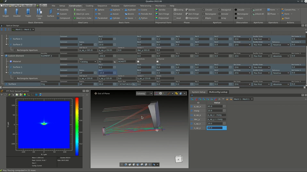
Now I will reduce the ray grid a bit so we can better see the elements Okay. So now since this is a parametric model, we can easily change some parameters.

And the first thing we can change, for example, is the aperture of this primary mirror.

Therefore, we just go here. We change the aperture to, let’s say, sixty five.

And you directly see the impact on the point spread function as well the rays being traced to the new design.

What we also can see here is that some rays get vignette it here, so we need to change this a bit, just increase the size here. So we’ll make it to twenty and fifteen.

And now we can see the mirror substrate is a bit too thin, so we will increase the thickness of the element here.

Okay. So this was my tutorial on the construction of this parametric design. I hope you enjoyed, and see you next time.