
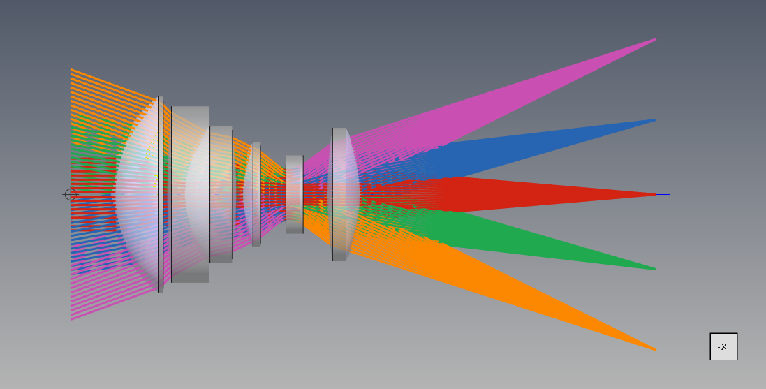
Designing optical systems frequently involves linking parameters or constraining them to achieve design specifications. These two tasks are implemented using what are commonly known as pickups and solves. Due to their importance in optical design, nearly all optical design software supports them in some form or another. Quadoa Optical CAD also supports these capabilities; however, the implementation is more flexible than most, enabling new functionality altogether.
PICKUPS
Pickups are used in optical systems design to link parameters having the same value, or a definable mathematical relationship between values. These are implemented in Quadoa by defining parameters and math functions in the Multi-Config Lookup table and using those values in the Optical Design editor. Let’s take a look at how this is done.
SIMPLE PICKUP
For cases where multiple parameters have the same value, a simple parameter is used in the multi-config table. A simple parameter is defined with an alphanumeric name (ID) and has the same value across any defined configurations. Go to File tab > Open Example and navigate to Basic Features\Telecentric_System.optx. This sample illustrates a doubly telecentric optical system using two lenses and an intermediate stop. Note the spacing between each lens and the stop is 100mm.
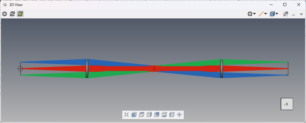
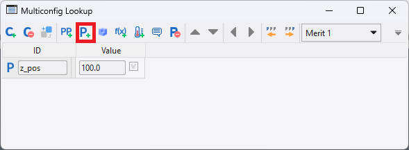
Go to Setup > Multi-Config to open the multi-configuration lookup table. In the toolbar of the multi-config table, select “P+” to create a new simple parameter. Give this parameter the ID name z_pos (this is arbitrary) and a Value of 100.
Once this simple parameter is defined, it can then be used in the Optical Design editor. Type the name of the parameter into the z-position cells for the stop surface (SURFACE 2) and the second lens (LENS 2).
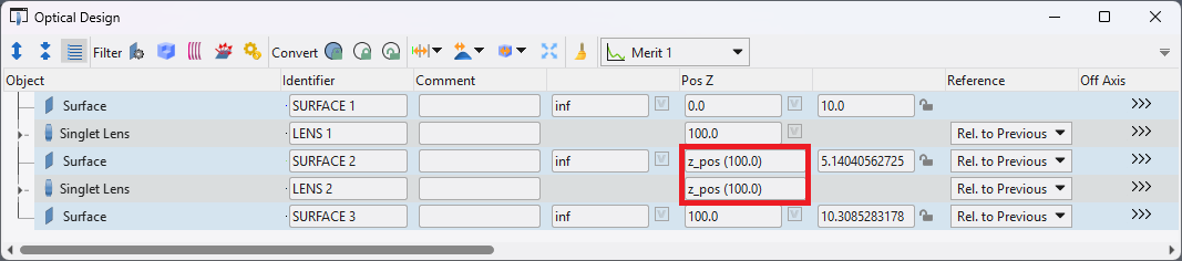
If done properly, the parameter name will display along with the current value in parentheses. If the goal is to optimize this value, its variable status can be activated next to the parameter definition in the multi-config lookup table. For reference, this is the same general method used to implement multi-config parameters using “PP+” (instead of “P+”).
COMPLEX PICKUP
The most basic math pickups support scaling and offsetting a parameter, providing an equation of the form P2 = SP1 + O, where S is a scale factor and O is an offset. In Quadoa, much more complex pickups are supported that allow arithmetic, trigonometric, and order of operation functions. By combining the simple parameters described previously with math expressions, a wide range of pickups are supported.
Open the sample file found under Examples\Objectives\Camera_Lens_75deg_FOV.optx.
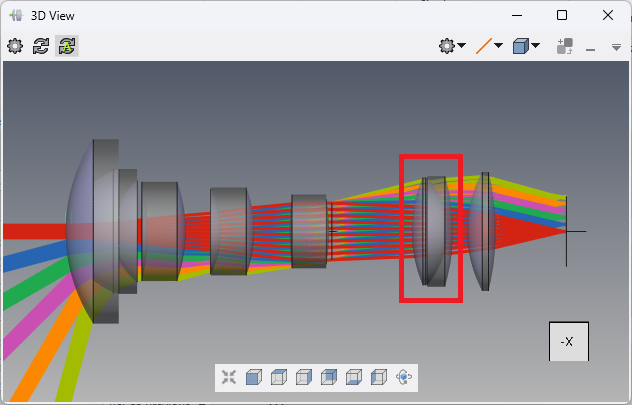
In this wide-angle camera objective, the doublet closest to the image plane is an air-spaced doublet. It may be desirable to link the radii of the two interior lens surfaces to ensure they have the same center of curvature, even as the spacing between them changes. To do this we would define two simple parameters as independent variables (first surface radius and surface spacing) and one math expression for the dependent variable (second surface radius). These are all defined in the multi-config lookup table. Copy the existing values for the radius and spacing to the lookup table. Then define the second radius as the difference of the first radius and the spacing.
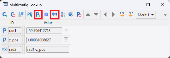
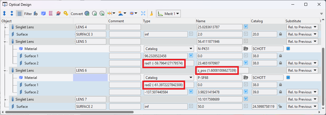
Once these parameters and math expression are defined, we then type them into the appropriate cells in the Optical Design editor. This implements a center of curvature pickup in our system.
For a more powerful illustration of the math pickup solve capability, take a look at the James Webb Space Telescope (JWST) sample file (Examples\Telescopes\JWST.optx). The position, asphere decenter, and curvature of each primary mirror segment is automatically calculated based upon the overall primary mirror aperture size and focal length. In addition, the slider tool defines an additional parameter used to simulate the deployment of the of the primary mirror.
SOLVES
Solves differ from pickups by optimizing one or more parameters to maintain a design constraint, typically based upon raytrace data. These are very useful in optical design and include constraints such as ray positions/angles, element power, first order properties, and more. In Quadoa, there are two types of solves: built-in solves and custom solves. Built-in solves are traditional solves on surface curvatures, component positions and orientations to align components to specific rays, foci or pupils. Custom solves can have arbitrary variables and goals, providing an extremely flexible automation tool.
BUILT-IN SOLVE
Let’s look at how we would implement a solve to maintain a surface centered upon and normal to an incident chief ray. Open the following sample file: Examples\Spectrometers\Spectrometer_With_Grating.optx.
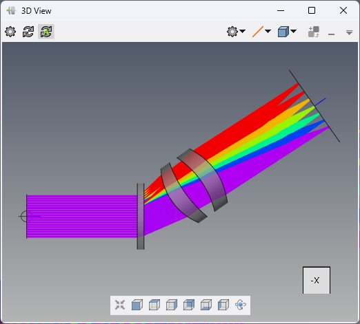
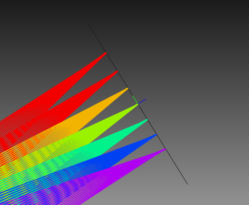
In this spectrometer sample file, a linear grating diffracts different wavelengths at different angles, which are then focused by a pair of lenses. Suppose we wanted to ensure that the image surface is centered on and normal to the central wavelength chief ray. We will need to define a solve on the y-position and x-rotation of the image surface.
In the Optical Design editor, navigate to the last surface (CAMERA) and notice the drop-down arrows next to the following parameters: Radius, Pos Z, Pos X, Pos Y, Rot X, Rot Y. Clicking this arrow will display the various solve options available.

Set the Pos Y and Rot X solves to “Align to Chief Ray”. Note that the image surface appears to align to the shortest wavelength chief ray. This is because solves default to operate on the primary wavelength (and on-axis field point). Go to the sequence definition and change the primary wavelength to wavelength number 4. Now you should see the image surface aligned to the central wavelength.
Built-in solves should be used instead of custom solves if they can achieve the desired constraint. They will update with every system update and can be utilized during optimization. They can also be used during tolerancing, however it is generally recommended to remove solves prior to tolerancing. This is because tolerancing is performed on a nominally fixed optical system that is being evaluated for manufacturing and assembly errors, and solves change the system from its nominal state.
CUSTOM SOLVES
When a built-in solve is not available to achieve a desired constraint, custom solves can be used. These solves are implemented as auto-applied merit functions that reoptimize with each system update. This is possible because Quadoa supports the simultaneous definition of multiple, independent merit functions. Note the “Auto-Apply” checkbox available on the top line of any merit function.
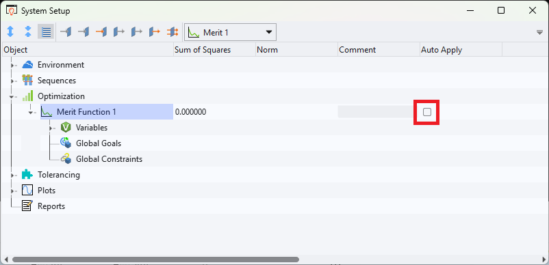
Using this method, any parameters and any calculated values available in the merit function can be utilized to create a custom solve. While the implementation of custom solves in Quadoa is flexible, it is important to keep in mind some guidelines. Because this merit function is optimized with each system update, it is critical that the variables be effective degrees of freedom and the goals be quick to compute. To enforce this, the optimizer will timeout after 1 second for auto-applied merit functions. Practically, custom solves cannot be used during optimization or tolerancing; they are not updated during these processes. They are intended to be used as design aids when manually setting up an optical system.
Quadoa Optical CAD provides flexible methods enabling custom parameter pickups or solves to be implemented.