Spot Radius Optimization

Transcription:

In this video, I will show you a simple optimization of an achromatic doublet. So you will see here the simple system, and you can find the system also under this name here in the example folder.

So before we start with our optimization, we have to define the variables which are allowed to be optimized by the optimizer.

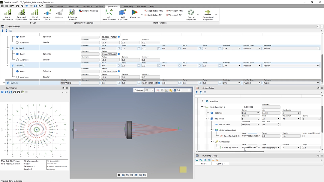
So for that, we go here to the optical design editor, and inside the optical design editor, we can see here these checkboxes.

And if I select here this checkbox, means that this parameter here, so in this case the radius of the surface one, is set as variable.

And I would like here to set the radius of the surface one, surface two, and also of the surface three as variable.

And for that, I will go here also to the radius of surface two and of surface three and select here the checkbox.

In addition, I will set here the focal length as variable as well because we define the focus by the numerical aperture.

In the next step, we will define the merit function. And to add a merit function, we can go here to the optimization tab and click here on the add merit function button.

Or we go here to the system setup, and we click here with the right mouse button on optimization and select here add a merit function.

So the merit function has been added here. If we open here the merit function, we see here the item ray trace.

And here we can select the sequence which should be optimized, and we can select the field which should be optimized. In my case, I would like to optimize all fields, and I would like to optimize all wavelengths.

And here you can select the configuration. So if you have defined the multi configuration, you can select the configuration which should be optimized.

So I click here with the right mouse button on the ray trace, and here we can add some aberration and optical property targets.

And I would like here to add the spot radius because I would like here to optimize my spot radius.

And if we open here the ray trace, we see that here under optimization goals, the spot radius has been added.

And here we can also weight my target. So if I have added here more than one target, we can weight them.

Here under constraints, I will click also with the right mouse button, and here we can add some aberration constraints and also optical property constraints.

And for my case, I will add here image space n a.

And if we open here the constraints, we see here this image space n a.

And here we can define, the target. So in my case, I would like to have an image space with zero point two or greater than this, and this should be a hard constraint by LaCroix.

Here on the bottom, we can see global constraints. So these are like mechanical constraints like center thickness and edge thickness.

So for the first, this should be okay for my merit function, and we will go here now to the local optimization.

And here we can select the merit function which which we would like to optimize. So in this case, merit merit function one because we have only one merit function.

And here we can select whether, my plots should be updated while optimizing.

So I click here. Okay.

Please update the three d view and the plots, and now I click here on optimize.

And what I see is right now that here my system has been optimized, and we see here in the spot diagram that the optimization has been done for all wavelengths here colored in different colors.

So the maximum radius is eighteen microns, and we see also that here my image space na, the value is zero point two as here defined as my target. So I showed you just a simple optimization, and thanks for watching.